What gives the confidence interval. Quantitative Analysis Methods: Estimating Confidence Intervals
Let's build a confidence interval in MS EXCEL for estimating the mean value of the distribution in the case known value dispersion.
Of course the choice level of trust completely depends on the task at hand. Thus, the degree of confidence of the air passenger in the reliability of the aircraft, of course, should be higher than the degree of confidence of the buyer in the reliability of the light bulb.
Task Formulation
Let's assume that from population having taken sample size n. It is assumed that standard deviation this distribution is known. Necessary on the basis of this samples evaluate the unknown distribution mean(μ, ) and construct the corresponding bilateral confidence interval.
Point Estimation
As is known from statistics(let's call it X cf) is an unbiased estimate of the mean this population and has the distribution N(μ;σ 2 /n).
Note: What if you need to build confidence interval in the case of distribution, which is not normal? In this case, comes to the rescue, which says that with enough big size samples n from distribution non- normal, sampling distribution of statistics Х av will approximately correspond normal distribution with parameters N(μ;σ 2 /n).
So, point estimate middle distribution values we have is sample mean, i.e. X cf. Now let's get busy confidence interval.
Building a confidence interval
Usually, knowing the distribution and its parameters, we can calculate the probability that a random variable will take a value from a given interval. Now let's do the opposite: find the interval in which the random variable falls with a given probability. For example, from properties normal distribution it is known that with a probability of 95%, a random variable distributed over normal law, will fall within the interval approximately +/- 2 from mean value(see article about). This interval will serve as our prototype for confidence interval.
Now let's see if we know the distribution , to calculate this interval? To answer the question, we must specify the form of distribution and its parameters.
We know the form of distribution is normal distribution(remember that we are talking about sampling distribution statistics X cf).
The parameter μ is unknown to us (it just needs to be estimated using confidence interval), but we have its estimate X cf, calculated based on sample, which can be used.
The second parameter is sample mean standard deviation will be known, it is equal to σ/√n.
Because we do not know μ, then we will build the interval +/- 2 standard deviations not from mean value, but from its known estimate X cf. Those. when calculating confidence interval we will NOT assume that X cf will fall within the interval +/- 2 standard deviations from μ with a probability of 95%, and we will assume that the interval is +/- 2 standard deviations from X cf with a probability of 95% will cover μ - the average of the general population, from which sample. These two statements are equivalent, but the second statement allows us to construct confidence interval.
In addition, we refine the interval: a random variable distributed over normal law, with a 95% probability falls within the interval +/- 1.960 standard deviations, not +/- 2 standard deviations. This can be calculated using the formula \u003d NORM.ST.OBR ((1 + 0.95) / 2), cm. sample file Sheet Spacing.

Now we can formulate a probabilistic statement that will serve us to form confidence interval:
"The probability that population mean located from sample average within 1.960" standard deviations of the sample mean", is equal to 95%.
The probability value mentioned in the statement has a special name , which is associated with significance level α (alpha) by a simple expression trust level =1 -α . In our case significance level α =1-0,95=0,05 .
Now, based on this probabilistic statement, we write an expression for calculating confidence interval:
where Zα/2 – standard normal distribution(such a value of a random variable z, what P(z>=Zα/2 )=α/2).
Note: Upper α/2-quantile defines the width confidence interval in standard deviations sample mean. Upper α/2-quantile standard normal distribution is always greater than 0, which is very convenient.
In our case, at α=0.05, upper α/2-quantile equals 1.960. For other significance levels α (10%; 1%) upper α/2-quantile Zα/2 can be calculated using the formula \u003d NORM.ST.OBR (1-α / 2) or, if known trust level, =NORM.ST.OBR((1+confidence level)/2).
Usually when building confidence intervals for estimating the mean use only upper α/2-quantile and do not use lower α/2-quantile. This is possible because standard normal distribution symmetrical about the x-axis ( density of its distribution symmetrical about average, i.e. 0). Therefore, there is no need to calculate lower α/2-quantile(it is simply called α /2-quantile), because it is equal upper α/2-quantile with a minus sign.
Recall that, regardless of the shape of the distribution of x, the corresponding random variable X cf distributed approximately fine N(μ;σ 2 /n) (see article about). Therefore, in general, the above expression for confidence interval is only approximate. If x is distributed over normal law N(μ;σ 2 /n), then the expression for confidence interval is accurate.
Calculation of confidence interval in MS EXCEL
Let's solve the problem.
The response time of an electronic component to an input signal is important characteristic devices. An engineer wants to plot a confidence interval for the average response time at a confidence level of 95%. From previous experience, the engineer knows that the standard deviation of the response time is 8 ms. It is known that the engineer made 25 measurements to estimate the response time, the average value was 78 ms.
Solution: Engineer wants to know the response time electronic device, but he understands that the response time is not fixed, but a random variable that has its own distribution. So the best he can hope for is to determine the parameters and shape of this distribution.
Unfortunately, from the condition of the problem, we do not know the form of the distribution of the response time (it does not have to be normal). , this distribution is also unknown. Only he is known standard deviationσ=8. Therefore, while we cannot calculate the probabilities and construct confidence interval.
However, although we do not know the distribution time separate response, we know that according to CPT, sampling distribution average response time is approximately normal(we will assume that the conditions CPT are performed, because size samples large enough (n=25)) .
Furthermore, the average this distribution is equal to mean value unit response distributions, i.e. μ. BUT standard deviation of this distribution (σ/√n) can be calculated using the formula =8/ROOT(25) .
It is also known that the engineer received point estimate parameter μ equal to 78 ms (X cf). Therefore, now we can calculate the probabilities, because we know the distribution form ( normal) and its parameters (Х ср and σ/√n).
Engineer wants to know expected valueμ of the response time distribution. As stated above, this μ is equal to expectation of the sample distribution of the average response time. If we use normal distribution N(X cf; σ/√n), then the desired μ will be in the range +/-2*σ/√n with a probability of approximately 95%.
Significance level equals 1-0.95=0.05.
Finally, find the left and right border confidence interval.
Left border: \u003d 78-NORM.ST.INR (1-0.05 / 2) * 8 / ROOT (25) =
74,864
Right border: \u003d 78 + NORM. ST. OBR (1-0.05 / 2) * 8 / ROOT (25) \u003d 81.136
Left border: =NORM.INV(0.05/2, 78, 8/SQRT(25))
Right border: =NORM.INV(1-0.05/2, 78, 8/SQRT(25))
Answer: confidence interval at 95% confidence level and σ=8msec equals 78+/-3.136ms
IN example file on sheet Sigma known created a form for calculation and construction bilateral confidence interval for arbitrary samples with a given σ and significance level.

CONFIDENCE.NORM() function
If the values samples are in the range B20:B79
, but significance level equal to 0.05; then MS EXCEL formula:
=AVERAGE(B20:B79)-CONFIDENCE(0.05,σ, COUNT(B20:B79))
will return the left border confidence interval.
The same boundary can be calculated using the formula:
=AVERAGE(B20:B79)-NORM.ST.INV(1-0.05/2)*σ/SQRT(COUNT(B20:B79))
Note: The TRUST.NORM() function appeared in MS EXCEL 2010. Earlier versions of MS EXCEL used the TRUST() function.
Confidence intervals ( English Confidence Intervals) one of the types of interval estimates used in statistics, which are calculated for a given level of significance. They allow us to make a statement that the true value of an unknown statistical parameter of the general population is in the obtained range of values with a probability that is given by the selected level. statistical significance.
Normal distribution
When the variance (σ 2 ) of the population of data is known, a z-score can be used to calculate confidence limits (boundary points of the confidence interval). Compared to using a t-distribution, using a z-score will not only provide a narrower confidence interval, but also provide more reliable estimates of the mean and standard deviation (σ), since the Z-score is based on a normal distribution.
Formula
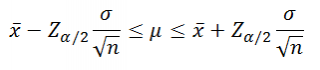
To determine the boundary points of the confidence interval, provided that the standard deviation of the population of data is known, the following formula is used
| L = X - Z α/2 | σ |
| √n |
Example
Assume that the sample size is 25 observations, the sample mean is 15, and the population standard deviation is 8. For a significance level of α=5%, the Z-score is Z α/2 =1.96. In this case, the lower and upper limits of the confidence interval will be
| L = 15 - 1.96 | 8 | = 11,864 |
| √25 |
| L = 15 + 1.96 | 8 | = 18,136 |
| √25 |
Thus, we can state that with a probability of 95% the mathematical expectation of the general population will fall in the range from 11.864 to 18.136.
Methods for narrowing the confidence interval
Let's say the range is too wide for the purposes of our study. There are two ways to decrease the confidence interval range.
- Reduce the level of statistical significance α.
- Increase the sample size.
Reducing the level of statistical significance to α=10%, we get a Z-score equal to Z α/2 =1.64. In this case, the lower and upper limits of the interval will be
| L = 15 - 1.64 | 8 | = 12,376 |
| √25 |
| L = 15 + 1.64 | 8 | = 17,624 |
| √25 |
And the confidence interval itself can be written as
In this case, we can make the assumption that with a probability of 90%, the mathematical expectation of the general population will fall into the range.
If we want to keep the level of statistical significance α, then the only alternative is to increase the sample size. Increasing it to 144 observations, we obtain the following values of the confidence limits
| L = 15 - 1.96 | 8 | = 13,693 |
| √144 |
| L = 15 + 1.96 | 8 | = 16,307 |
| √144 |
The confidence interval itself will look like this:
Thus, narrowing the confidence interval without reducing the level of statistical significance is only possible by increasing the sample size. If it is not possible to increase the sample size, then the narrowing of the confidence interval can be achieved solely by reducing the level of statistical significance.
Building a confidence interval for a non-normal distribution
If the standard deviation of the population is not known or the distribution is non-normal, the t-distribution is used to construct a confidence interval. This technique is more conservative, which is expressed in wider confidence intervals, compared to the technique based on the Z-score.
Formula
The following formulas are used to calculate the lower and upper limits of the confidence interval based on the t-distribution
| L = X - tα | σ |
| √n |
Student's distribution or t-distribution depends on only one parameter - the number of degrees of freedom, which is equal to the number of individual feature values (the number of observations in the sample). The value of Student's t-test for a given number of degrees of freedom (n) and the level of statistical significance α can be found in the lookup tables.
Example
Assume that the sample size is 25 individual values, the mean value of the sample is 50, and the standard deviation of the sample is 28. You need to construct a confidence interval for the level of statistical significance α=5%.
In our case, the number of degrees of freedom is 24 (25-1), therefore, the corresponding tabular value of Student's t-test for the level of statistical significance α=5% is 2.064. Therefore, the lower and upper bounds of the confidence interval will be
| L = 50 - 2.064 | 28 | = 38,442 |
| √25 |
| L = 50 + 2.064 | 28 | = 61,558 |
| √25 |
And the interval itself can be written as
Thus, we can state that with a probability of 95% the mathematical expectation of the general population will be in the range.
Using a t-distribution allows you to narrow the confidence interval, either by reducing statistical significance or by increasing the sample size.
Reducing the statistical significance from 95% to 90% in the conditions of our example, we get the corresponding tabular value of Student's t-test 1.711.
| L = 50 - 1.711 | 28 | = 40,418 |
| √25 |
| L = 50 + 1.711 | 28 | = 59,582 |
| √25 |
In this case, we can say that with a probability of 90% the mathematical expectation of the general population will be in the range.
If we do not want to reduce the statistical significance, then the only alternative is to increase the sample size. Let's say that it is 64 individual observations, and not 25 as in the initial condition of the example. The tabular value of Student's t-test for 63 degrees of freedom (64-1) and the level of statistical significance α=5% is 1.998.
| L = 50 - 1.998 | 28 | = 43,007 |
| √64 |
| L = 50 + 1.998 | 28 | = 56,993 |
| √64 |
This gives us the opportunity to assert that with a probability of 95% the mathematical expectation of the general population will be in the range.
Large Samples
Large samples are samples from a population of data with more than 100 individual observations. Statistical studies have shown that larger samples tend to be normally distributed, even if the distribution of the population is not normal. In addition, for such samples, the use of z-score and t-distribution give approximately the same results when constructing confidence intervals. Thus, for large samples, it is acceptable to use a z-score for a normal distribution instead of a t-distribution.
Summing up
"Katren-Style" continues to publish a cycle of Konstantin Kravchik on medical statistics. In two previous articles, the author touched on the explanation of such concepts as and.
Konstantin Kravchik
Mathematician-analyst. Specialist in the field of statistical research in medicine and humanities
Moscow city
Very often in articles on clinical trials you can find a mysterious phrase: "confidence interval" (95% CI or 95% CI - confidence interval). For example, an article might say: "Student's t-test was used to assess the significance of differences, with a 95% confidence interval calculated."
What is the value of the "95% confidence interval" and why calculate it?
What is a confidence interval? - This is the range in which the true mean values in the population fall. And what, there are "untrue" averages? In a sense, yes, they do. In we explained that it is impossible to measure the parameter of interest in the entire population, so the researchers are content with a limited sample. In this sample (for example, by body weight) there is one average value (a certain weight), by which we judge the average value in the entire general population. However, hardly average weight in a sample (especially a small one) will coincide with the average weight in the general population. Therefore, it is more correct to calculate and use the range of average values of the general population.
For example, suppose the 95% confidence interval (95% CI) for hemoglobin is between 110 and 122 g/L. This means that with a 95 % probability, the true mean value for hemoglobin in the general population will be in the range from 110 to 122 g/l. In other words, we do not know average hemoglobin in the general population, but we can indicate the range of values for this feature with 95% probability.
Confidence intervals are particularly relevant to the difference in means between groups, or what is called the effect size.
Suppose we compared the effectiveness of two iron preparations: one that has been on the market for a long time and one that has just been registered. After the course of therapy, the concentration of hemoglobin in the studied groups of patients was assessed, and the statistical program calculated for us that the difference between the average values of the two groups with a probability of 95% is in the range from 1.72 to 14.36 g/l (Table 1).
Tab. 1. Criterion for independent samples
(groups are compared by hemoglobin level)
This should be interpreted as follows: in a part of patients in the general population who take a new drug, hemoglobin will be higher on average by 1.72–14.36 g/l than in those who took an already known drug.
In other words, in the general population, the difference in the average values for hemoglobin in groups with a 95% probability is within these limits. It will be up to the researcher to judge whether this is a lot or a little. The point of all this is that we are not working with one average value, but with a range of values, therefore, we more reliably estimate the difference in a parameter between groups.
In statistical packages, at the discretion of the researcher, one can independently narrow or expand the boundaries of the confidence interval. By lowering the probabilities of the confidence interval, we narrow the range of means. For example, at 90% CI, the range of means (or mean differences) will be narrower than at 95% CI.
Conversely, increasing the probability to 99% widens the range of values. When comparing groups, the lower limit of the CI may cross the zero mark. For example, if we extended the boundaries of the confidence interval to 99 %, then the boundaries of the interval ranged from –1 to 16 g/L. This means that in the general population there are groups, the difference between the averages between which for the studied trait is 0 (M=0).
Confidence intervals can be used to test statistical hypotheses. If the confidence interval crosses zero, then the null hypothesis, which assumes that the groups do not differ in the studied parameter, is true. An example is described above, when we expanded the boundaries to 99%. Somewhere in the general population, we found groups that did not differ in any way.
95% confidence interval of difference in hemoglobin, (g/l)

The figure shows the 95% confidence interval of the mean hemoglobin difference between the two groups as a line. The line passes the zero mark, therefore, there is a difference between the average values, zero, which confirms the null hypothesis that the groups do not differ. The difference between the groups ranges from -2 to 5 g/l, which means that hemoglobin can either decrease by 2 g/l or increase by 5 g/l.
Confidence interval - very important indicator. Thanks to it, you can see if the differences in the groups were really due to the difference in the means or due to a large sample, because with a large sample, the chances of finding differences are greater than with a small one.
In practice, it might look like this. We took a sample of 1000 people, measured the hemoglobin level and found that the confidence interval for the difference in the means lies from 1.2 to 1.5 g/L. The level of statistical significance in this case p
We see that the hemoglobin concentration increased, but almost imperceptibly, therefore, the statistical significance appeared precisely due to the sample size.
Confidence intervals can be calculated not only for averages, but also for proportions (and risk ratios). For example, we are interested in the confidence interval of the proportions of patients who achieved remission while taking the developed drug. Assume that the 95% CI for the proportions, i.e. for the proportion of such patients, is in the range 0.60–0.80. Thus, we can say that our medicine has a therapeutic effect in 60 to 80% of cases.
The analysis of random errors is based on the theory of random errors, which makes it possible, with a certain guarantee, to calculate the actual value of the measured quantity and evaluate possible errors.
The basis of the theory of random errors is the following assumptions:
with a large number of measurements, random errors of the same magnitude, but of a different sign, occur equally often;
large errors are less common than small ones (the probability of an error decreases with an increase in its value);
with an infinitely large number of measurements, the true value of the measured quantity is equal to the arithmetic mean of all measurement results;
the appearance of one or another measurement result as a random event is described by the normal distribution law.
In practice, a distinction is made between a general and a sample set of measurements.
Under the general population
imply the whole set of possible measurement values or possible error values  .
.
For sample population
number of measurements  limited, and in each case strictly defined. They think that if
  , then the average value of this set of measurements
  close enough to its true value.
1. Interval Estimation Using Confidence Probability
For a large sample and a normal distribution law, the general evaluation characteristic of the measurement is the variance  and coefficient of variation
  :
:
 ;
;
 .
(1.1)
.
(1.1)
Dispersion characterizes the homogeneity of a measurement. The higher  , the greater the measurement scatter.
The coefficient of variation characterizes variability. The higher  , the greater the variability of the measurements relative to the mean values.
To assess the reliability of measurement results, the concepts of confidence interval and confidence probability are introduced into consideration.
Trusted
is called the interval
values  ,
in which the true value falls
,
in which the true value falls  measured quantity with a given probability.
Confidence Probability
(reliability) of a measurement is the probability that the true value of the measured quantity falls within a given confidence interval, i.e. to the zone  . This value is determined in fractions of a unit or in percent.
 ,
,
where  - integral Laplace function ( table 1.1
)
- integral Laplace function ( table 1.1
)
The integral Laplace function is defined by the following expression:
 .
.
The argument to this function is guarantee factor :
Table 1.1
Integral Laplace function

If, on the basis of certain data, a confidence probability is established  (often taken to be
  ), then set accuracy of measurements
(confidence interval
), then set accuracy of measurements
(confidence interval
 ) based on the ratio
 .
.
Half of the confidence interval is
 ,
(1.3)
,
(1.3)
where  - argument of the Laplace function, if
  (table 1.1
);
(table 1.1
);
 - Student's functions, if
  (table 1.2
).
(table 1.2
).
Thus, the confidence interval characterizes the measurement accuracy of a given sample, and the confidence level characterizes the measurement reliability.
Example
Done  measurements of the strength of the road surface of the site highway with an average modulus of elasticity
  and the calculated value of the standard deviation
  .
.
Necessary determine the required accuracy measurements for different levels confidence level  , taking the values
  on table 1.1
.
on table 1.1
.
In this case, respectively |
Therefore, for a given measurement tool and method, the confidence interval increases by about  times if you increase
  just on
  .
.
Confidence intervals.
The calculation of the confidence interval is based on the average error of the corresponding parameter. Confidence interval shows within what limits with probability (1-a) is the true value of the estimated parameter. Here a is the significance level, (1-a) is also called the confidence level.
In the first chapter, we showed that, for example, for the arithmetic mean, the true population mean lies within 2 mean errors of the mean about 95% of the time. Thus, the boundaries of the 95% confidence interval for the mean will be from the sample mean by twice the mean error of the mean, i.e. we multiply the mean error of the mean by some factor that depends on the confidence level. For the mean and the difference of the means, the Student's coefficient (the critical value of the Student's criterion) is taken, for the share and difference of the shares, the critical value of the z criterion. The product of the coefficient and the average error can be called the marginal error of this parameter, i.e. the maximum that we can get when evaluating it.
Confidence interval for arithmetic mean : .
Here is the sample mean;
Average error of the arithmetic mean;
s- sample standard deviation;
n
f = n-1 (Student's coefficient).
Confidence interval for difference of arithmetic means :
Here, is the difference between the sample means;
 - the average error of the difference of arithmetic means;
s 1 ,s 2 - sample standard deviations;
n1,n2
Critical value of the Student's criterion for a given level of significance a and the number of degrees of freedom f=n1 +n2-2 (Student's coefficient).
Confidence interval for shares :
![]() .
.
Here d is the sample share;
– average share error;
n– sample size (group size);
Confidence interval for share differences :
Here, is the difference between the sample shares;
 is the mean error of the difference between the arithmetic means;
n1,n2– sample sizes (number of groups);
The critical value of the criterion z at a given significance level a ( , , ).
By calculating the confidence intervals for the difference in indicators, we, firstly, directly see the possible values of the effect, and not just its point estimate. Secondly, we can draw a conclusion about the acceptance or refutation of the null hypothesis and, thirdly, we can draw a conclusion about the power of the criterion.
When testing hypotheses using confidence intervals, one must adhere to next rule:
If the 100(1-a)-percent confidence interval of the mean difference does not contain zero, then the differences are statistically significant at the a significance level; on the contrary, if this interval contains zero, then the differences are not statistically significant.
Indeed, if this interval contains zero, then, it means that the compared indicator can be either more or less in one of the groups compared to the other, i.e. the observed differences are random.
By the place where zero is located within the confidence interval, one can judge the power of the criterion. If zero is close to the lower or upper limit of the interval, then perhaps with a larger number of compared groups, the differences would reach statistical significance. If zero is close to the middle of the interval, then it means that both increase and decrease of the indicator in experimental group, and there probably aren't really any differences.
Examples:
To compare operational lethality when using two different types of anesthesia: 61 people were operated on using the first type of anesthesia, 8 died, using the second - 67 people, 10 died.
d 1 \u003d 8/61 \u003d 0.131; d 2 \u003d 10/67 \u003d 0.149; d1-d2 = - 0.018.
The difference in lethality of the compared methods will be in the range (-0.018 - 0.122; -0.018 + 0.122) or (-0.14; 0.104) with a probability of 100(1-a) = 95%. The interval contains zero, i.e. hypothesis about the same mortality in two different types anesthesia cannot be denied.
Thus, mortality can and will decrease to 14% and increase to 10.4% with a probability of 95%, i.e. zero is approximately in the middle of the interval, so it can be argued that, most likely, these two methods really do not differ in lethality.
In the example considered earlier, the average tapping time was compared in four groups of students differing in their examination scores. Let's calculate the confidence intervals of the average pressing time for students who passed the exam for 2 and 5 and the confidence interval for the difference between these averages.
Student's coefficients are found from the tables of Student's distribution (see Appendix): for the first group: = t(0.05;48) = 2.011; for the second group: = t(0.05;61) = 2.000. Thus, confidence intervals for the first group: = (162.19-2.011 * 2.18; 162.19 + 2.011 * 2.18) = (157.8; 166.6) , for the second group (156.55- 2.000*1.88 ; 156.55+2.000*1.88) = (152.8 ; 160.3). So, for those who passed the exam for 2, the average pressing time ranges from 157.8 ms to 166.6 ms with a probability of 95%, for those who passed the exam for 5 - from 152.8 ms to 160.3 ms with a probability of 95%.
You can also test the null hypothesis using confidence intervals for the means, and not just for the difference in the means. For example, as in our case, if the confidence intervals for the means overlap, then the null hypothesis cannot be rejected. In order to reject a hypothesis at a chosen significance level, the corresponding confidence intervals must not overlap.
Let's find the confidence interval for the difference in the average pressing time in the groups who passed the exam for 2 and 5. The difference in the averages: 162.19 - 156.55 = 5.64. Student's coefficient: \u003d t (0.05; 49 + 62-2) \u003d t (0.05; 109) \u003d 1.982. Group standard deviations will be equal to: ; . We calculate the average error of the difference between the means: . Confidence interval: \u003d (5.64-1.982 * 2.87; 5.64 + 1.982 * 2.87) \u003d (-0.044; 11.33).
So, the difference in the average pressing time in the groups that passed the exam at 2 and at 5 will be in the range from -0.044 ms to 11.33 ms. This interval includes zero, i.e. the average pressing time for those who passed the exam with excellent results can both increase and decrease compared to those who passed the exam unsatisfactorily, i.e. the null hypothesis cannot be rejected. But zero is very close to the lower limit, the time of pressing is much more likely to decrease for excellent passers. Thus, we can conclude that there are still differences in the average click time between those who passed by 2 and by 5, we just could not detect them for a given change in the average time, the spread of the average time and sample sizes.
The power of the test is the probability of rejecting an incorrect null hypothesis, i.e. find differences where they really are.
The power of the test is determined based on the level of significance, the magnitude of differences between groups, the spread of values in groups, and the sample size.
For Student's t-test and analysis of variance, you can use sensitivity charts.
The power of the criterion can be used in the preliminary determination of the required number of groups.
The confidence interval shows within what limits the true value of the estimated parameter lies with a given probability.
With the help of confidence intervals, you can test statistical hypotheses and draw conclusions about the sensitivity of the criteria.
LITERATURE.
Glantz S. - Chapter 6.7.
Rebrova O.Yu. - p.112-114, p.171-173, p.234-238.
Sidorenko E. V. - pp. 32-33.
Questions for self-examination of students.
1. What is the power of the criterion?
2. In what cases is it necessary to evaluate the power of criteria?
3. Methods for calculating power.
6. How to test a statistical hypothesis using a confidence interval?
7. What can be said about the power of the criterion when calculating the confidence interval?
Tasks.